Textbooks (Including Mine) Are a Little Wrong about Interrupted Time Series

Underdog method that nobody is actually rooting for takes another one on the chin.

“Interrupted time series,” like many terms in statistical analysis, has many meanings.¹ But here I mean a research design in which case you look at an event that occurred at a specific point in time. To estimate the effect of that event on some outcome Y, you estimate a time series of Y in the time leading up to the event, and another time series of Y in the time following the event. The change in that time series from just before the event to just after is the effect of treatment. See that link for more detail.

A common, basic, way of implementing an interrupted time series is with regression. In the linear case you might run a model like this:

\(Y_t = \beta_0 + \beta_1t + \beta_2After_t + \beta_3t\times After_t + \varepsilon_t\)

Where t is a variable for the time period, usually adjusted for convenience such that the last period before the event occurs is t = 0. After is a binary variable equal to t > 0. If we are in the “post-event” period, After is 1. In the “pre-event” period, After is 0. ε is an error term.

This model is easily extensible to allow for non-linear trends, such as in this quadratic/parabolic model:

\(Y_t = \beta_0 + \beta_{1a}t + \beta_{2b}t^2 + \beta_2After_t + \beta_{3a}t\times After_t + \beta_{3b}t^2 \times After_t + \varepsilon_t\)

These models look very similar to the regression model you might use to estimate a regression discontinuity design, when using linear regression to implement that design. And indeed the intuition is similar: we want to compare a predicted outcome just to one side of a cutoff (just before the event) to just on the other side of the cutoff (just after the event).²

So what’s the issue, then? No problem so far.

Interpretation

One positive feature of the interrupted time series model is how easy it is to interpret. Just like with other cases where we have an interaction term, we can interpret the result by taking its derivative. Want to know the effect of the event? Well, you’re looking at the case of going from After = 0 to After = 1 while holding the rest constant, or the effect of a one-unit change in After.

Want the effect of a change in one variable on another? Take a derivative! Still the best advice I have for interpreting interaction terms.³ In the linear model:

\(\frac{\partial Y}{\partial After} = \beta_2 + \beta_3t\)

and in the quadratic:

\(\frac{\partial Y}{\partial After} = \beta_2 + \beta_{3a}t + \beta_{3b}t^2\)

Since we have an interaction, the effect of After obviously differs across different values of t. However, we’re interested in the point where the event goes into effect. Remember how we adjusted t so that point was at t = 0? That means we want the effect of After at t = 0. Which is nice and easy! All those t terms drop out and we’re left with the effect simply being:

\(\frac{\partial Y}{\partial After}|(t=0) = \beta_2\)

for both the linear model and the quadratic version (and the cubic, and quartic, and so on).

Interrupted time series leaves us with the nice convenient result that the immediate effect of the event, adjusted for time trends on either side, is a single coefficient easily located on the regression table. This is the interpretation you’ll see in my textbook,⁴ and from many other people as well.

Indeed, that’s the same interpretation we have when using this equation for regression discontinuity - the effect of treatment is just the coefficient on “being above the cutoff.” And this article isn’t about a problem in regression discontinuity.⁵ What’s different for interrupted time series?

What is Zero Anyway?

The problem arises because of the thing we said we wanted to estimate. We said, just like if we were doing regression discontinuity, that we wanted the effect of After at the point t = 0. We’re in calculus-world here (remember the derivative?) meaning that we want the impact of switching from Before to After at the infinitesimal moment where it occurs. That’s what we’re asking the regression to calculate when we just look at β2 as the effect.

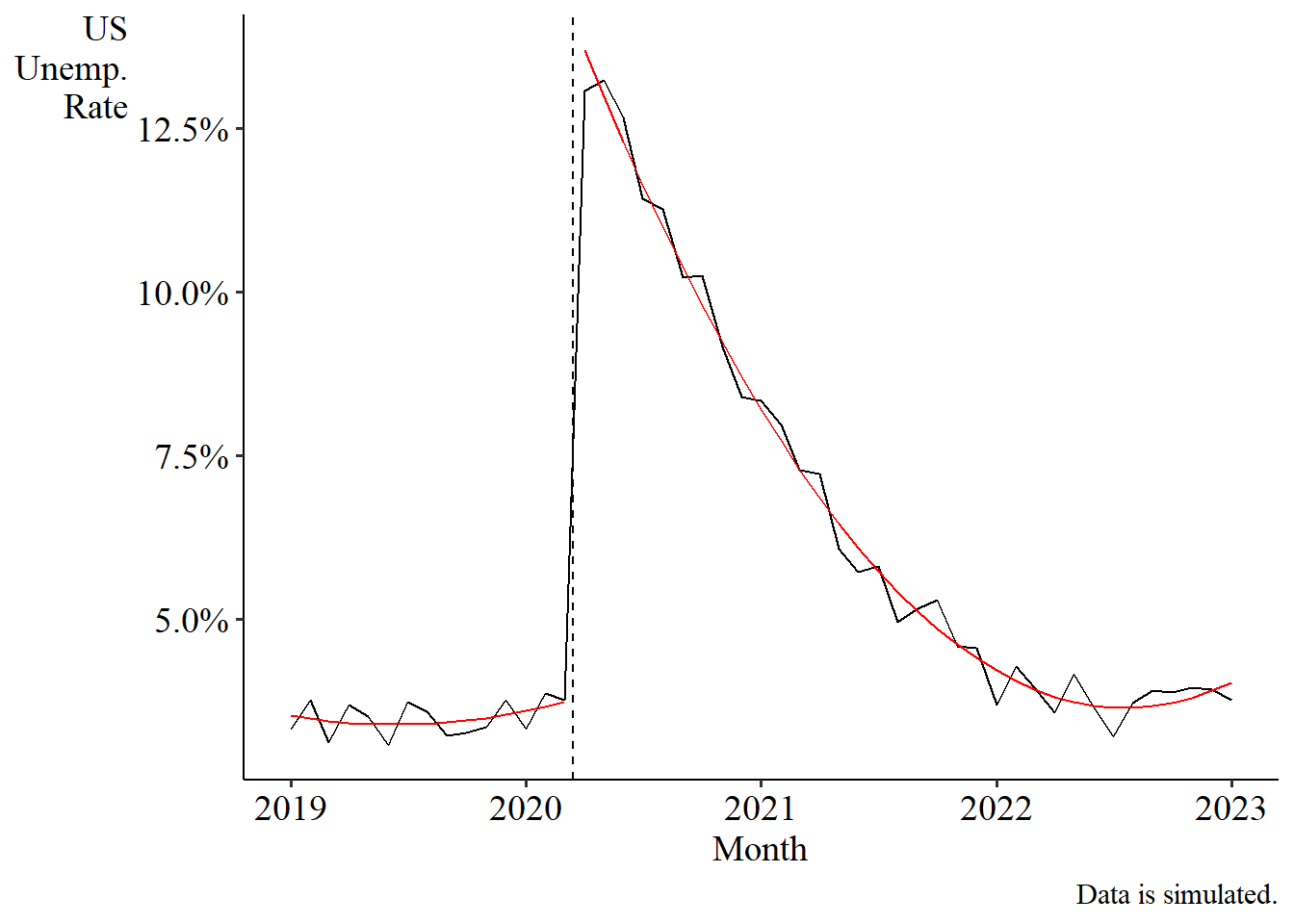
But is that actually what we want? Well, the real-world example that inspired this article was looking at the effect of COVID on the US unemployment rate. You can see the problem in that data, but here’s some simulated data that isolates the issue more cleanly. Here’s what the data looks like:

If we eyeball the effect, it looks like the unemployment rate rose by about 10 percentage points at the onset of COVID. Indeed, in data I actually generated, the “true” effect that I baked in was 10 percentage points, and after adding noise, the jump from March to April 2020 is 9.3 percentage points.

Great. Let’s estimate an interrupted time series. There’s clearly some sort of curve on the right side; looks parabola-esque (I did literally enforce a quadratic data generating process here, but the real data looks like this too!). So let’s fit a quadratic model.

                                     m
Dependent Var.:                 UNRATE
                                      
Constant            0.0374*** (0.0020)
t                      0.0008 (0.0007)
AfterTRUE           0.1071*** (0.0026)
t square             4.67e-5 (4.63e-5)
t x AfterTRUE      -0.0084*** (0.0007)
AfterTRUE x I(t^2)  8.56e-5. (4.67e-5)
__________________ ___________________
S.E. type                          IID
Observations                        49
R2                             0.99107
Adj. R2                        0.99003
---
Signif. codes: 0 '***' 0.001 '**' 0.01 '*' 0.05 '.' 0.1 ' ' 1

The model tells us that the effect of COVID on unemployment was 10.7 percentage points (the coefficient on AfterTRUE). That’s meaningfully above the actual jump in the data of 9.3 percentage points, and is even meaningfully above the “true” effect of 10 percentage points.

What’s happening? Well, when we eyeball the data, we’re imagining two time trends that look something like this:

And, indeed, those are the regression fits from the model! And this looks reasonable. Perhaps that single point in April 2020 is a bit below the curve, but not that much. And… this matches our eyeball result, more or less. The jump from March to April 2020 is not the 10.7 percentage points we got from the regression table, but rather a flat 10.0 percentage points - the true jump I baked into the data! But we get something more than that, 10.7, in our regression estimate.

So why don’t we get the eyeball result? Why is the eyeball result closer to the truth than the regression result? Heck, why are the regression predictions closer to the truth than the… estimate from the regression model that’s supposed to represent the same thing?

Because the After coefficient is not based on a jump from t = 0 to t = 1, like what we see in that graph. It’s based on an infinitesimal jump from t = 0 to t = 0! In other words, we have to extend that parabola all the way back to t = 0 to see the effect:

Oh.

The difference between the eyeball result, and even the regression-prediction result, and the regression coefficient result, happens because the red line keeps moving even after the data stops. The red line on the right was already keening up a little too high as we move from right to left and meet that April 2020 point. But as we keep moving left, the red line, our regression model result, keeps going even after the black line, our eyeball result, stops.

The problem occurs because, in many event study applications, the question “what changed from just before to just after” means “from the period just before to the period just after”. But in our calculus-based interpretation, it instead means “at the period just before”.⁶

In any data where your time series shows a large slope near the event period, and your time periods cover fairly long windows, like a month, or a year, the difference between these two ideas can become quite severe! (And in fact if you repeat this exercise using actual unemployment data, you’ll get worse results using quarterly unemployment than monthly, or if you repeat it without that big ol’ slope right after the event, the problem goes away). In some cases you might trust your functional form enough to believe its extrapolation back to t = 0 and think that you want that particular interpretation. But I suspect in many interrupted time series cases that’s not actually what you want.

The Fix

The fix here is quite easy: just do a calculation that matches the interpretation you are going for, which is “from the period just before to the period just after”, or in other words get the predicted value at t = 1 and subtract out the predicted value at t = 0. Conveniently, this isn’t too difficult either. Just… don’t hold t fixed when going from before to after! Let it increase by 1 unit as well. This gives us, in the linear case:

\(E(Y|t=1) - E(Y|t = 0) = \beta_0 + \beta_1 + \beta_2After + \beta_3After - \beta_0\)

and when we note that After = 1 when t = 1, this simplifies to an effect of

\(E(Y|t=1) - E(Y|t = 0) = \beta_1+\beta_2+\beta_3\)

Not too bad! Similar math shows us that the equivalent effect in the quadratic model is just

\(E(Y|t=1) - E(Y|t = 0) = \beta_{1a} + \beta_{1b}+\beta_2+\beta_{3a}+\beta_{3b}\)

So just add up everything but the intercept! Not too hard.

Applying this quadratic form to our COVID unemployment model gives us an effect of 0.09967, just about bang on the 10-percentage-point truth.

Conclusion

If you want something discrete, do something discrete! If you don’t, don’t. All shall be well.

1. I claimed literally last night (as I write this on Friday) that my next Substack post would be a YouTube video. But then I got this idea. So the next one will be a YouTube video. I’m a maverick. A loose cannon. I don’t play by the rules.

2. Interrupted time series results are generally considered weaker than regression discontinuity results, if only because the RDD assumption that the only thing changing from one side of the cutoff to another is treatment is more plausible when, say, comparing a test score of 79.9 vs. a test score of 80.1, than comparing one month to the next month, where by the sheer nature of the passage of time many things are likely to change. If you prefer (although I’d definitely disagree with your terminology) you could say “RDD with time as a running variable is weaker than RDD with other running variables”. But hey, what are you gonna do? The regression equations do at least look similar.

3. True, technically the derivative doesn’t exist here because After is binary, but this all seems to just sorta work anyway for interaction terms. Crucially, the extent to which this might be mathematically imprecise or wrong is not the wrong thing I’m pointing out in this article, and in my opinion is more or less just fine.

4. Although I will consider adding a note about this in the next edition.

5. Although, to be fair, you can construct examples where a similar problem occurs for RDD done with OLS. The RDD literature usually discusses this in the context of worrying about functional form (or sometimes granularity of the running variable, or the combination of the two).

6. Usually, regression discontinuity wants this latter interpretation, so the same issue doesn’t happen there.